How common is it to have no academic weaknesses?

I’m afraid that the question posed by the title does not have a single answer. It depends on how we define and measure academic performance.

Let’s sidestep some difficult questions about what exactly an “academic deficit” is and for the sake of convenience pretend that it is a score at least 1 standard deviation below the mean on a well normed test administered by a competent psychologist with good clinical skills.

Suppose that we start with the 9 core WJ III achievement tests (the answers will not be all that different with the new WJ IV):

	Reading	Writing	Mathematics
Skills	Letter-Word Identification	Spelling	Calculation
Applications	Passage Comprehension	Writing Samples	Applied Problems
Fluency	Reading Fluency	Writing Fluency	Math Fluency

What is the percentage of the population that does not have any score below 85? If we can assume that the scores are multivariate normal, the answer can be found using data simulation or via the cumulative density function of the multivariate normal distribution. I gave examples of both methods in the previous post. If we use the correlation matrix for the 6 to 9 age group of the WJ III NU, about 47% of the population has no academic scores below 85.

Using the same methods we can estimate what percent of the population has no academic scores below various thresholds. Subtracting these numbers from 100%, we can see that fairly large proportions have at least one low score.

Threshold	% with no scores below the threshold	% with at least one score below the threshold
85	47%	53%
80	63%	37%
75	77%	23%
70	87%	13%

What proportion of people with average cognitive scores have no academic weaknesses?

The numbers in the table above include people with very low cognitive ability. It would be more informative if we could control for a person’s measured cognitive abilities.

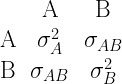
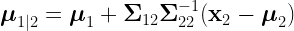
Suppose that an individual has index scores of exactly 100 for all 14 subtests that are used to calculate the WJ III GIA Extended. We can calculate the means and the covariance matrix of the achievement tests for all people with this particular cognitive profile. We will make use of the conditional multivariate normal distribution. As explained here (or here), we partition the academic tests $(\mathbf{X}_1)$ and the cognitive predictor tests $(\mathbf{X}_2)$ like so:

$\begin{pmatrix}\mathbf{X}_1 \\ \mathbf{X}_2 \end{pmatrix}\sim\mathcal{N}\left(\begin{pmatrix}\boldsymbol{\mu}_1 \\ \boldsymbol{\mu}_2\end{pmatrix},\begin{pmatrix}\mathbf{\Sigma}_{11} & \mathbf{\Sigma}_{12} \\ \mathbf{\Sigma}_{21} & \mathbf{\Sigma}_{22}\end{pmatrix}\right)$

$\boldsymbol{\mu}_1$ and $\boldsymbol{\mu}_2$ are the mean vectors for the academic and cognitive variables, respectively.
$\mathbf{\Sigma}_{11}$ and $\mathbf{\Sigma}_{22}$ are the covariances matrices of academic and cognitive variables, respectively.
$\mathbf{\Sigma}_{12}$ is the matrix of covariances between the academic and cognitive variables.

If the cognitive variables have the vector of particular values $\mathbf{x}_2$ , then the conditional mean vector of the academic variables $(\boldsymbol{\mu}_{1|2})$ is:

$\boldsymbol{\mu}_{1|2}=\boldsymbol{\mu}_1+\mathbf{\Sigma}_{12}\mathbf{\Sigma}^{-1}_{22}(\mathbf{x}_2-\boldsymbol{\mu}_2)$

The conditional covariance matrix:
$\mathbf{\Sigma}_{1|2}=\mathbf{\Sigma}_{11}-\mathbf{\Sigma}_{12}\mathbf{\Sigma}^{-1}_{22}\mathbf{\Sigma}_{21}$

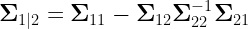
If we can assume multivariate normality, we can use these equations, to estimate the proportion of people with no scores below any threshold on any set of scores conditioned on any set of predictor scores. In this example, about 51% of people with scores of exactly 100 on all 14 cognitive predictors have no scores below 85 on the 9 academic tests. About 96% of people with this cognitive profile have no scores below 70.

Because there is an extremely large number of possible cognitive profiles, I cannot show what would happen with all of them. Instead, I will show what happens with all of the perfectly flat profiles from all 14 cognitive scores equal to 70 to all 14 cognitive scores equal to 130.

What proportion of people with flat WJ III cognitive profiles equal to 70 to 130 have no WJ III academic scores below 85

Here is what happens with the same procedure when the threshold is 70 for the academic scores:

What proportion of people with flat WJ III cognitive profiles equal to 70 to 130 have no WJ III academic scores below 70

Here is the R code I used to perform the calculations. You can adapt it to other situations fairly easily (different tests, thresholds, and profiles).

library(mvtnorm)
WJ <- matrix(c(
  1,0.49,0.31,0.46,0.57,0.28,0.37,0.77,0.36,0.15,0.24,0.49,0.25,0.39,0.61,0.6,0.53,0.53,0.5,0.41,0.43,0.57,0.28, #Verbal Comprehension
  0.49,1,0.27,0.32,0.47,0.26,0.32,0.42,0.25,0.21,0.2,0.41,0.21,0.28,0.38,0.43,0.31,0.36,0.33,0.25,0.29,0.4,0.18, #Visual-Auditory Learning
  0.31,0.27,1,0.25,0.33,0.18,0.21,0.28,0.13,0.16,0.1,0.33,0.13,0.17,0.25,0.22,0.18,0.21,0.19,0.13,0.25,0.31,0.11, #Spatial Relations
  0.46,0.32,0.25,1,0.36,0.17,0.26,0.44,0.19,0.13,0.26,0.31,0.18,0.36,0.4,0.36,0.32,0.29,0.31,0.27,0.22,0.33,0.2, #Sound Blending
  0.57,0.47,0.33,0.36,1,0.29,0.37,0.49,0.28,0.16,0.23,0.57,0.24,0.35,0.4,0.44,0.36,0.38,0.4,0.34,0.39,0.53,0.27, #Concept Formation
  0.28,0.26,0.18,0.17,0.29,1,0.35,0.25,0.36,0.17,0.27,0.29,0.53,0.22,0.37,0.32,0.52,0.42,0.32,0.49,0.42,0.37,0.61, #Visual Matching
  0.37,0.32,0.21,0.26,0.37,0.35,1,0.3,0.24,0.13,0.22,0.33,0.21,0.35,0.39,0.34,0.38,0.38,0.36,0.33,0.38,0.43,0.36, #Numbers Reversed
  0.77,0.42,0.28,0.44,0.49,0.25,0.3,1,0.37,0.15,0.23,0.43,0.23,0.37,0.56,0.55,0.51,0.47,0.47,0.39,0.36,0.51,0.26, #General Information
  0.36,0.25,0.13,0.19,0.28,0.36,0.24,0.37,1,0.1,0.22,0.21,0.38,0.26,0.26,0.33,0.4,0.28,0.27,0.39,0.21,0.25,0.32, #Retrieval Fluency
  0.15,0.21,0.16,0.13,0.16,0.17,0.13,0.15,0.1,1,0.06,0.16,0.17,0.09,0.11,0.09,0.13,0.1,0.12,0.13,0.07,0.12,0.07, #Picture Recognition
  0.24,0.2,0.1,0.26,0.23,0.27,0.22,0.23,0.22,0.06,1,0.22,0.35,0.2,0.16,0.22,0.25,0.21,0.19,0.26,0.17,0.19,0.21, #Auditory Attention
  0.49,0.41,0.33,0.31,0.57,0.29,0.33,0.43,0.21,0.16,0.22,1,0.2,0.3,0.33,0.38,0.29,0.31,0.3,0.25,0.42,0.47,0.25, #Analysis-Synthesis
  0.25,0.21,0.13,0.18,0.24,0.53,0.21,0.23,0.38,0.17,0.35,0.2,1,0.15,0.19,0.22,0.37,0.21,0.2,0.4,0.23,0.19,0.37, #Decision Speed
  0.39,0.28,0.17,0.36,0.35,0.22,0.35,0.37,0.26,0.09,0.2,0.3,0.15,1,0.39,0.36,0.32,0.3,0.3,0.3,0.25,0.33,0.23, #Memory for Words
  0.61,0.38,0.25,0.4,0.4,0.37,0.39,0.56,0.26,0.11,0.16,0.33,0.19,0.39,1,0.58,0.59,0.64,0.5,0.48,0.46,0.52,0.42, #Letter-Word Identification
  0.6,0.43,0.22,0.36,0.44,0.32,0.34,0.55,0.33,0.09,0.22,0.38,0.22,0.36,0.58,1,0.52,0.52,0.47,0.42,0.43,0.49,0.36, #Passage Comprehension
  0.53,0.31,0.18,0.32,0.36,0.52,0.38,0.51,0.4,0.13,0.25,0.29,0.37,0.32,0.59,0.52,1,0.58,0.48,0.65,0.42,0.43,0.59, #Reading Fluency
  0.53,0.36,0.21,0.29,0.38,0.42,0.38,0.47,0.28,0.1,0.21,0.31,0.21,0.3,0.64,0.52,0.58,1,0.5,0.49,0.46,0.47,0.49, #Spelling
  0.5,0.33,0.19,0.31,0.4,0.32,0.36,0.47,0.27,0.12,0.19,0.3,0.2,0.3,0.5,0.47,0.48,0.5,1,0.44,0.41,0.46,0.36, #Writing Samples
  0.41,0.25,0.13,0.27,0.34,0.49,0.33,0.39,0.39,0.13,0.26,0.25,0.4,0.3,0.48,0.42,0.65,0.49,0.44,1,0.38,0.37,0.55, #Writing Fluency
  0.43,0.29,0.25,0.22,0.39,0.42,0.38,0.36,0.21,0.07,0.17,0.42,0.23,0.25,0.46,0.43,0.42,0.46,0.41,0.38,1,0.57,0.51, #Calculation
  0.57,0.4,0.31,0.33,0.53,0.37,0.43,0.51,0.25,0.12,0.19,0.47,0.19,0.33,0.52,0.49,0.43,0.47,0.46,0.37,0.57,1,0.46, #Applied Problems
  0.28,0.18,0.11,0.2,0.27,0.61,0.36,0.26,0.32,0.07,0.21,0.25,0.37,0.23,0.42,0.36,0.59,0.49,0.36,0.55,0.51,0.46,1), nrow= 23, byrow=TRUE) #Math Fluency
WJNames <- c("Verbal Comprehension", "Visual-Auditory Learning", "Spatial Relations", "Sound Blending", "Concept Formation", "Visual Matching", "Numbers Reversed", "General Information", "Retrieval Fluency", "Picture Recognition", "Auditory Attention", "Analysis-Synthesis", "Decision Speed", "Memory for Words", "Letter-Word Identification", "Passage Comprehension", "Reading Fluency", "Spelling", "Writing Samples", "Writing Fluency", "Calculation", "Applied Problems", "Math Fluency")
rownames(WJ) <- colnames(WJ) <- WJNames

#Number of tests
k<-length(WJNames)

#Means and standard deviations of tests
mu<-rep(100,k)
sd<-rep(15,k)

#Covariance matrix
sigma<-diag(sd)%*%WJ%*%diag(sd)
colnames(sigma)<-rownames(sigma)<-WJNames

#Vector identifying predictors (WJ Cog)
p<-seq(1,14)

#Threshold for low scores
Threshold<-85

#Proportion of population who have no scores below the threshold
pmvnorm(lower=rep(Threshold,length(WJNames[-p])),upper=rep(Inf,length(WJNames[-p])),sigma=sigma[-p,-p],mean=mu[-p])[1]

#Predictor test scores for an individual
x<-rep(100,length(p))
names(x)<-WJNames[p]

#Condition means and covariance matrix
condMu<-c(mu[-p] + sigma[-p,p] %*% solve(sigma[p,p]) %*% (x-mu[p]))
condSigma<-sigma[-p,-p] - sigma[-p,p] %*% solve(sigma[p,p]) %*% sigma[p,-p]

#Proportion of people with the same predictor scores as this individual who have no scores below the threshold
pmvnorm(lower=rep(Threshold,length(WJNames[-p])),upper=rep(Inf,length(WJNames[-p])),sigma=condSigma,mean=condMu)[1]

Cognitive Assessment, Psychometrics, Statistics

How unusual is it to have multiple scores below a threshold?

In psychological assessment, it is common to specify a threshold at which a score is considered unusual (e.g., 2 standard deviations above or below the mean). If we can assume that the scores are roughly normal, it is easy to estimate the proportion of people with scores below the threshold we have set. If the threshold is 2 standard deviations below the mean, then the Excel function NORMSDIST will tell us the answer:

=NORMSDIST(-2)

=0.023

In R, the pnorm function gives the same answer:

pnorm(-2)

How unusual is it to have multiple scores below the threshold? The answer depends on how correlated the scores are. If we can assume that the scores are multivariate normal, Crawford and colleagues (2007) show us how to obtain reasonable estimates using simulated data. Here is a script in R that depends on the mvtnorm package. Suppose that the 10 subtests of the WAIS-IV have correlations as depicted below. Because the subtests have a mean of 10 and a standard deviation of 3, the scores are unusually low if 4 or lower.

#WAIS-IV subtest names
WAISSubtests <- c("BD", "SI", "DS", "MR", "VO", "AR", "SS", "VP", "IN", "CD")

# WAIS-IV correlations
WAISCor <- rbind(
  c(1.00,0.49,0.45,0.54,0.45,0.50,0.41,0.64,0.44,0.40), #BD
  c(0.49,1.00,0.48,0.51,0.74,0.54,0.35,0.44,0.64,0.41), #SI
  c(0.45,0.48,1.00,0.47,0.50,0.60,0.40,0.40,0.43,0.45), #DS
  c(0.54,0.51,0.47,1.00,0.51,0.52,0.39,0.53,0.49,0.45), #MR
  c(0.45,0.74,0.50,0.51,1.00,0.57,0.34,0.42,0.73,0.41), #VO
  c(0.50,0.54,0.60,0.52,0.57,1.00,0.37,0.48,0.57,0.43), #AR
  c(0.41,0.35,0.40,0.39,0.34,0.37,1.00,0.38,0.34,0.65), #SS
  c(0.64,0.44,0.40,0.53,0.42,0.48,0.38,1.00,0.43,0.37), #VP
  c(0.44,0.64,0.43,0.49,0.73,0.57,0.34,0.43,1.00,0.34), #IN
  c(0.40,0.41,0.45,0.45,0.41,0.43,0.65,0.37,0.34,1.00)) #CD
rownames(WAISCor) <- colnames(WAISCor) <- WAISSubtests

#Means
WAISMeans<-rep(10,length(WAISSubtests))

#Standard deviations
WAISSD<-rep(3,length(WAISSubtests))

#Covariance Matrix
WAISCov<-WAISCor*WAISSD%*%t(WAISSD)

#Sample size
SampleSize<-1000000

#Load mvtnorm package
library(mvtnorm)

#Make simulated data
d<-rmvnorm(n=SampleSize,mean=WAISMeans,sigma=WAISCov)
#To make this more realistic, you can round all scores to the nearest integer (d<-round(d))

#Threshold for abnormality
Threshold<-4

#Which scores are less than or equal to threshold
Abnormal<- d<=Threshold

#Number of scores less than or equal to threshold
nAbnormal<-rowSums(Abnormal)

#Frequency distribution table
p<-c(table(nAbnormal)/SampleSize)

#Plot
barplot(p,axes=F,las=1,
    xlim=c(0,length(p)*1.2),ylim=c(0,1),
    bty="n",pch=16,col="royalblue2",
    xlab="Number of WAIS-IV subtest scores less than or equal to 4",
    ylab="Proportion")
axis(2,at=seq(0,1,0.1),las=1)
text(x=0.7+0:10*1.2,y=p,labels=formatC(p,digits=2),cex=0.7,pos=3,adj=0.5)

The code produces this graph:

Using the multivariate normal distribution

The simulation method works very well, especially if the sample size is very large. An alternate method that gives more precise numbers is to estimate how much of the multivariate normal distribution is within certain bounds. That is, we find all of the regions of the multivariate normal distribution in which one and only one test is below a threshold and then add up all the probabilities. The process is repeated to find all regions in which two and only two tests are below a threshold. Repeat the process, with 3 tests, 4 tests, and so on. This is tedious to do by hand but only takes a few lines of code do automatically.

AbnormalPrevalance<-function(Cor,Mean=0,SD=1,Threshold){
  require(mvtnorm)
  k<-nrow(Cor)
  p<-rep(0,k)
  zThreshold<-(Threshold-Mean)/SD
  for (n in 1:k){
    combos<-combn(1:k,n)
    ncombos<-ncol(combos)
    for (i in 1:ncombos){
      u<-rep(Inf,k)
      u[combos[,i]]<-zThreshold
      l<-rep(-Inf,k)
      l[seq(1,k)[-combos[,i]]]<-zThreshold 
      p[n]<-p[n]+pmvnorm(lower=l,upper=u,mean=rep(0,k),sigma=Cor)[1]
    }
  }
  p<-c(1-sum(p),p)
  names(p)<-0:k

  barplot(p,axes=F,las=1,xlim=c(0,length(p)*1.2),ylim=c(0,1),
     bty="n",pch=16,col="royalblue2",
     xlab=bquote("Number of scores less than or equal to " * .(Threshold)),
     ylab="Proportion")
  axis(2,at=seq(0,1,0.1),las=1)
  text(x=0.7+0:10*1.2,y=p,labels=formatC(p,digits=2),cex=0.7,pos=3,adj=0.5)
  return(p)
}
Proportions<-AbnormalPrevalance(Cor=WAISCor,Mean=10,SD=3,Threshold=4)

Using this method, the results are nearly the same but slightly more accurate. If the number of tests is large, the code can take a long time to run.

Cognitive Assessment, Psychometrics, R, Statistics, Tutorial

Using the multivariate truncated normal distribution

In a previous post, I imagined that there was a gifted education program that had a strictly enforced selection procedure: everyone with an IQ of 130 or higher is admitted. With the (univariate) truncated normal distribution, we were able to calculate the mean of the selected group (mean IQ = 135.6).

Multivariate Truncated Normal Distributions

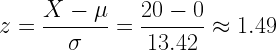
Reading comprehension has a strong relationship with IQ $(\rho\approx 0.70)$ . What is the average reading comprehension score among students in the gifted education program? If we can assume that reading comprehension is normally distributed $(\mu=100, \sigma=15)$ and the relationship between IQ and reading comprehension is linear $(\rho=0.70)$ , then we can answer this question using the multivariate truncated normal distribution. Portions of the multivariate normal distribution have been truncated (sliced off). In this case, the blue portion of the bivariate normal distribution of IQ and reading comprehension has been sliced off. The portion remaining (in red), is the distribution we are interested in. Here it is in 3D:

Bivariate normal distribution truncated at IQ = 130

Here is the same distribution with simulated data points in 2D:

Truncated bivariate normal distribution with simulated data

Expected values of IQ and reading comprehension when IQ ≥ 130

Expected Values

In the picture above, the expected value (i.e., mean) for the IQ of the students in the gifted education program is 135.6. In the last post, I showed how to calculate this value.

The expected value (i.e., mean) for the reading comprehension score is 124.9. How is this calculated? The general method is fairly complicated and requires specialized software such as the R package tmvtnorm. However in the bivariate case with a single truncation, we can simply calculate the predicted reading comprehension score when IQ is 135.6:

$\dfrac{\hat{Y}-\mu_Y}{\sigma_Y}=\rho_{XY}\dfrac{X-\mu_X}{\sigma_X}$

$\dfrac{\hat{Y}-100}{15}=0.7\dfrac{135.6-100}{15}$

$\hat{Y}=124.9$

In R, the same answer is obtained via the tmvtnorm package:

library(tmvtnorm)
#Variable names
vNames<-c("IQ","Reading Comprehension")

#Vector of Means
mu<-c(100,100)
names(mu)<-vNames;mu

#Vector of Standard deviations
sigma<-c(15,15)
names(sigma)<-vNames;sigma

#Correlation between IQ and Reading Comprehension
rho<-0.7

#Correlation matrix
R<-matrix(c(1,rho,rho,1),ncol=2)
rownames(R)<-colnames(R)<-vNames;R

#Covariance matrix
C<-diag(sigma)%*%R%*%diag(sigma)
rownames(C)<-colnames(C)<-vNames;C

#Vector of lower bounds (-Inf means negative infinity)
a<-c(130,-Inf)

#Vector of upper bounds (Inf means positive infinity)
b<-c(Inf,Inf)

#Means and covariance matrix of the truncated distribution
m<-mtmvnorm(mean=mu,sigma=C,lower=a,upper=b)
rownames(m$tvar)<-colnames(m$tvar)<-vNames;m

#Means of the truncated distribution
tmu<-m$tmean;tmu

#Standard deviations of the truncated distribution
tsigma<-sqrt(diag(m$tvar));tsigma

#Correlation matrix of the truncated distribution
tR<-cov2cor(m$tvar);tR

In running the code above, we learn that the standard deviation of reading comprehension has shrunk from 15 in the general population to 11.28 in the truncated population. In addition, the correlation between IQ and reading comprehension has shrunk from 0.70 in the general population to 0.31 in the truncated population.

Marginal cumulative distributions

Among the students in the gifted education program, what proportion have reading comprehension scores of 100 or less? The question can be answered with the marginal cumulative distribution function. That is, what proportion of the red truncated region is less than 100 in reading comprehension? Assuming that the code in the previous section has been run already, this code will yield the answer of about 1.3%:

#Proportion of students in the gifted program with reading comprehension of 100 or less
ptmvnorm(lowerx=c(-Inf,-Inf),upperx=c(Inf,100),mean=mu,sigma=C,lower=a,upper=b)

The mean, sigma, lower, and upper parameters define the truncated normal distribution. The lowerx and the upperx parameters define the lower and upper bounds of the subregion in question. In this case, there are no restrictions except an upper limit of 100 on the second axis (the Y-axis).

If we plot the cumulative distribution of reading comprehension scores in the gifted population, it is close to (but not the same as) that of the conditional distribution of reading comprehension at IQ = 135.6.

Marginal cumulative distribution function of the truncated bivariate normal distribution

What proportion does the truncated distribution occupy in the untruncated distribution?

Imagine that in order to qualify for services for intellectual disability, a person must score 70 or below on an IQ test. Every three years, the person must undergo a re-evaluation. Suppose that the correlation between the original test and the re-evaluation test is $\rho=0.90$ . If the entire population were given both tests, what proportion would score 70 or lower on both tests? What proportion would score below 70 on the first test but not on the second test? Such questions can be answered with the pmvnorm function from the mvtnorm package (which is a prerequiste of the tmvtnorm package and this thus already loaded if you ran the previous code blocks).

library(mvtnorm)
#Means
IQmu<-c(100,100)

#Standard deviations
IQsigma<-c(15,15)

#Correlation
IQrho<-0.9

#Correlation matrix
IQcor<-matrix(c(1,IQrho,IQrho,1),ncol=2)

#Covariance matrix
IQcov<-diag(IQsigma)%*%IQcor%*%diag(IQsigma)

#Proportion of the general population scoring 70 or less on both tests
pmvnorm(lower=c(-Inf,-Inf),upper=c(70,70),mean=IQmu,sigma=IQcov)

#Proportion of the general population scoring 70 or less on the first test but not on the second test
pmvnorm(lower=c(-Inf,70),upper=c(70,Inf),mean=IQmu,sigma=IQcov)

What are the means of these truncated distributions?

#Mean scores among people scoring 70 or less on both tests
mtmvnorm(mean=IQmu,sigma=IQcov,lower=c(-Inf,-Inf),upper=c(70,70))

#Mean scores among people scoring 70 or less on the first test but not on the second test
mtmvnorm(mean=IQmu,sigma=IQcov,lower=c(-Inf,70),upper=c(70,Inf))

Combining this information in a plot:

Thus, we can see that the multivariate truncated normal distribution can be used to answer a wide variety of questions. With a little creativity, we can apply it to many more kinds of questions.

My Software & Spreadsheets, Psychometrics, Statistics

Using the truncated normal distribution

The term truncated normal distribution may sound highly technical but it is actually fairly simple and has many practical applications. If the math below is daunting, be assured that it is not necessary to understand the notation and the technical details. I have created a user-friendly spreadsheet that performs all the calculations automatically.

The mean of a truncated normal distribution

Imagine that your school district has a gifted education program. All students in the program have an IQ of 130 or higher. What is the average IQ of this group? Assume that in your school district, IQ is normally distributed with a mean of 100 and a standard deviation of 15.

Questions like this one can be answered by calculating the mean of the truncated normal distribution. The truncated normal distribution is a normal distribution in which one or both ends have been sliced off (i.e., truncated). In this case, everything below 130 has been sliced off (and there is no upper bound).

Four parameters determine the properties of the truncated normal distribution:

μ = mean of the normal distribution (before truncation)
σ = standard deviation of the normal distribution (before truncation)
a = the lower bound of the distribution (can be as low as −∞)
b = the upper bound of the distribution (can be as high as +∞)

The formula for the mean of a truncated distribution is a bit of a mess but can be simplified by finding the z-scores associated with the lower and upper bounds of the distribution:

$z_a=\dfrac{a-\mu}{\sigma}$

$z_b=\dfrac{b-\mu}{\sigma}$

The expected value of the truncated distribution (i.e., the mean):
$E(X)=\mu+\sigma\dfrac{\phi(z_a)-\phi(z_b)}{\Phi(z_b)-\Phi(z_a)}$

Where $\phi$ is the probability density function of the standard normal distribution (NORMDIST(z,0,1,FALSE) in Excel, dnorm(z) in R) and $\Phi$ is the cumulative distribution function of the standard normal distribution (NORMSDIST(z) in Excel, pnorm(z) in R).

This spreadsheet calculates the mean (and standard deviation) of a truncated distribution. See the part below the plot that says “Truncated Normal Distribution.”

In R you could make a function to calculate the mean of a truncated distribution like so:

MeanNormalTruncated<-function(mu=0,sigma=1,a=-Inf,b=Inf){
  mu+sigma*(dnorm((a-mu)/sigma)-dnorm((b-mu)/sigma))/(pnorm((b-mu)/sigma)-pnorm((a-mu)/sigma))
}

#Example: Find the mean of a truncated normal distribution with a mu = 100, sigma = 15, and lower bound = 130
MeanNormalTruncated(mu=100,sigma=15,a=130)

The cumulative distribution function of the truncated normal distribution

Suppose that we wish to know the proportion of students in the same gifted education program who score 140 or more. The cumulative truncated normal distribution function tells us the proportion of the distribution that is less than a particular value.

$cdf=\dfrac{\Phi(z_x)-\Phi(z_a)}{\Phi(z_b)-\Phi(z_a)}$

Where $z_x = \dfrac{X-\mu}{\sigma}$

In the previously mentioned spreadsheet, the cumulative distribution function is the proportion of the shaded region that is less than the value you specify.

You can create your own cumulative distribution function for the truncated normal distribution in R like so:

cdfNormalTruncated<-function(x=0,mu=0,sigma=1,a=-Inf,b=Inf){
  (pnorm((x-mu)/sigma)-pnorm((a-mu)/sigma))/(pnorm((b-mu)/sigma)-pnorm((a-mu)/sigma))
}
#Example: Find the proportion of the distribution less than 140
cdfNormalTruncated(x=140,mu=100,sigma=15,a=130)

In this case, the cumulative distribution function returns approximately 0.8316. Subtracting from 1, gives the proportion of scores 140 and higher: 0.1684. This means that about 17% of students in the gifted program can be expected to have IQ scores of 140 or more.¹

The truncated normal distribution in R

A fuller range of functions related to the truncated normal distribution can be found in the truncnorm package in R, including the expected value (mean), variance, pdf, cdf, quantile, and random number generation functions.

1 In the interest of precision, I need to say that because IQ scores are rounded to the nearest integer, a slight adjustment needs to be made. The true lower bound of the truncated distribution is not 130 but 129.5. Furthermore, we want the proportion of scores 139.5 and higher, not 140 and higher. This means that the expected proportion of students with IQ scores of “140” and higher in the gifted program is about 0.1718 instead of 0.1684. Of course, there is little difference between these estimates and such precision is not usually needed for “back-of-the-envelope” estimates such as this one.

Psychometrics

Reliability is where the light is. Validity is where the keys are.

There is a tired old joke about the drunk who lost his keys on the dark side of the street but is looking for them under the lamppost because “That’s where the light is.”

Reliability is where the light is. Validity is where the keys are.

Reliability is relatively easy to estimate compared to validity. Researchers and test developers make a very big deal out of high reliability coefficients because “A test cannot be valid if it is not reliable.” However, the fact that a measure is highly reliable is irrelevant if it does not allow us to make accurate inferences about the thing we wish to measure. Furthermore, if a measure is shown to have validity, its reliability is already implied.

To switch metaphors, reliability is thin gruel if validity is on the table. I think that with good models such as those offered by Weiss and colleagues (2013), validity is at least on the menu, if not already laid out for the feast. Reliability is at best an appetizer. It is nice to have, but if the main course is ample, you can skip it without worries.

This post is an excerpt from:

Schneider, W. J. (2013). What if we took our models seriously? Estimating latent scores in individuals. Journal of Psychoeducational Assessment, 31, 186–201.

Psychometrics, Statistics

Viewing correlation from a different angle

The typical way that we display correlated data is that we plot the points on an X–Y plane. The data are correlated to the degree to which the points are contained within a narrow, slanted ellipse.

Correlation with Orthogonal Axes

I believe that this is, in fact, the most intuitive way to display correlated data. However, there is an alternate way of doing it that yields interesting insights.

Oblique Axes

In the plot above, the X and Y axes are orthogonal (at a right angle). However, we can make scatterplots in which the axes are oblique (not orthogonal). This is hard to think about at first but after a while it makes sense. No matter what, the points are at the intersection of two vectors perpendicular to the axes. For example, point A (2,2) and point B (1,3) can be displayed with oblique axes like so:

Orthogonal vs. Oblique Axes

If we make the cosine of the angle between X and Y axes to equal the correlation coefficient, something interesting happens. Suppose that X and Y are normally distributed z-scores with a correlation of 0.8. When the cosine of the angle between the axes equals the correlation coefficient, the data appear to be contained in a circle rather than in an ellipse.

Correlated data with oblique axes

What is the value of this way of looking at correlations? There are many insights to be had but for now I will focus on two. First, partially correlated data are partially redundant. Viewing the data with oblique axes gives us an alternate way of seeing how redundant the information provided by the two variables is. Second, viewing the data with oblique axes gives an idea as to what is happening with principal components analysis.

Oblique Axes and Principal Components Analysis

Principal components analysis takes our data and summarizes it in the most economical way possible. With only 2 correlated variables, the first principal component is a summary of overall elevation of the 2 scores. If X and Y both equal 2 (and the correlation is 0.8), the score on the first principal component is about 2.11 (which, like all composite scores, is slightly more extreme than the weighted average of its parts).

In the plot above, the first principal component (PC₁) is the red vector that bisects X and Y. The cosine of the angle between PC₁ and the X-axis is X’s correlation with PC₁ (also known as X’s loading on PC₁). Because there are only two variables, X and Y have equal loadings on PC₁.

The second principal component (PC₂) is orthogonal to the first principal component. The meaning of PC₂ depends on how many variables there are and their structure. In the case of two positively correlated variables, PC₂ is a summary of the magnitude of the difference between the scores. If X = 2 and Y = 1, they differ by 1 standard score. If X and Y are highly correlated, this is a large difference and the score on PC₂ would be large. If X and Y have a low correlation, this difference is not so large and the score on PC₂ is more modest.

Oblique Axes and the Mahalanobis Distance

The Mahalanobis distance is a measure of how unusual a profile of scores is in a particular population. Shown with oblique axes, the Mahalanobis distance is simply the distance of the point to the origin (at the population mean). Suppose that X and Y have correlation of 0.90. As shown below, if X is 1 standard deviation above the mean and Y is 1 standard deviations below the mean, the Mahalanobis distance for this point is going to be large (4.5).

For multivariate k normal variables, the Mahalanobis distance has a χ distribution with k degrees of freedom (the χ distribution occurs when you take the square root of every value in the more well known χ² distribution). In the χ distribution with 2 degrees of freedom, a value of 4.5 is greater than 99.95% of values. Thus, (-1,1) is a quite unusual pair of scores if the z-scores correlate at ρ = 0.90

Mahalanobis Distance of an atypical set of scores

If both X and Y are 1 standard deviation above the mean, the Mahalanobis distance would be fairly small (1.03). In the χ distribution with 2 degrees of freedom, a value of 1.03 is greater than only 39% of values, making this a fairly typical pair of scores.

More typical scores

Psychometrics, Statistics

Difference scores, the absolute deviation, and the half-normal distribution

In psychological assessment, sometimes we want to contrast two scores. For example, suppose we give two tests of visual-spatial ability to an individual. On Test A the score was 95 and on Test B the score was 75.

Two tests of visual-spatial ability differ by 20 points.

Both tests are measured with the index score metric (mean = 100, SD = 15). Because these tests are intended to measure the same ability, we are surprised to see that they differ by 20 points (20 index score points = 1⅓ standard deviations). How common is it for tests that allegedly measure the same thing to differ by 20 points or more?

The answer, of course, depends on the distributions of both variables and the form of the relationship between the two variables. In this case, let’s assume that the tests are multivariate normal, meaning that both variables have normal distributions and any linear combination of the two scores (included subtracting the scores) is also normal.

A Bivariate Normal Distribution with a correlation of 0.6

The relationship between the two variables is linear. Linear relationships are fully described by correlation coefficients. In this case, suppose that the correlation coefficient is 0.6.

Few variables found in nature have a true multivariate normal distribution. However, multivariate normal distributions describe cognitive ability data reasonably well.

The mean of a difference score

The mean of the sum of two variables is the sum of the two means. That is,

$\mu_{A + B} = \mu_A + \mu_B=100+100=200$

It works the same way with subtraction:

$\mu_{A - B} = \mu_A - \mu_B=100-100=0$

The standard deviation of a difference score

The standard deviation of the sum of two variables is the square root of the sum of the two variables’ covariance matrix. The covariance matrix is:

$\begin{matrix} & \text{A} & \text{B} \\ \text{A} & \sigma_A^2 & \sigma_{AB} \\ \text{B} & \sigma_{AB} & \sigma_B^2 \end{matrix}$

The sum of the covariance matrix is:

$\sigma_{A+B}=\sqrt{ \sigma_{A}^2 + 2\sigma_{AB} + \sigma_{B}^2}$

The covariance is the product of the two standard deviations and the correlation (ρ):

$\sigma_{AB}=\sigma_A \sigma_B \rho_{AB}$

Thus,

$\sigma_{A+B}=\sqrt{15^2+2*15*15*0.6+15^2}\approx 26.83$

The standard deviation of the difference of two variables is the same except that the covariance is negative.

$\sigma_{A-B}=\sqrt{ \sigma_{A}^2 - 2\sigma_{AB} + \sigma_{B}^2}$

$\sigma_{A-B}=\sqrt{15^2-2*15*15*0.6+15^2}\approx13.42$

The prevalence of a difference score

If the two variables are multivariate normal, then the difference score is also normally distributed. The difference of A and B in this example is:

$A-B=95-75=20$

The population mean of the difference scores is 0 and the standard deviation is 13.24.

Using the z-score formula,

$z=\dfrac{X-\mu}{\sigma}=\dfrac{20-0}{13.42}\approx 1.49$

The cumulative distribution function of the standard normal distribution (Φ) is the proportion of scores to the left of a particular z-score. In Excel, the Φ function is the NORMSDIST function.

$\Phi(1.49)=\texttt{NORMSDIST}(1.49)\approx 0.93$

Thus about 7% (1−0.93=0.07) of people have a difference score of 20 or more in this particular direction and about 14% have difference score of 20 or more in either direction. Thus, in this case, a difference of 20 points or more is only somewhat unusual.

The absolute deviation

The standard deviation is a sort of average deviation but it is not the arithmetic mean of the deviations. If you really want to know the average (unsigned) deviation, then you want the absolute deviation. Technically, the absolute deviation is the expected value of the absolute value of the deviation:

$\text{Absolute Deviation}=E(|X-\mu|)$

Sometimes the absolute deviation is the calculated as the average deviation from the median instead of from the mean. In the case of the normal distribution, this difference does not matter because the mean and median are the same.

In the normal distribution, the absolute deviation is about 80% as large as the standard deviation. Specifically,

$\text{Absolute Deviation}=\sqrt{\dfrac{2}{\pi}}\sigma$

The absolute deviation of a difference score

If the two variables are multivariate normal, the difference score is also normal. We calculate the standard deviation of the difference score and multiply it by the square root of 2 over pi. In this case, the standard deviation of the difference score was about 13.42. Thus, the average difference score is:

$\sqrt{\dfrac{2}{\pi}}13.42\approx 10.70$

Why use the absolute deviation?

The standard deviation is the standard way of describing variability. Why would we use this obscure type of deviation then? Well, most people have not heard of either kind of deviation. For people who have never taken a statistics course, it is very easy to talk about the average difference score (i.e., the absolute deviation). For example, “On average, these two scores differ by 11 points.” See how easy that was?

In contrast, imagine saying to statistically untrained people, “The standard deviation is the square root of the average squared difference from the population mean. In this case it is 13 points.” Sure, this explanation can be made simpler…but at the expense of accuracy.

The absolute deviation can be explained easily AND accurately.

The half-normal distribution

Related to the idea of the absolute deviation is the half-normal distribution. The half-normal distribution occurs when we take a normally distributed variable and take the absolute value of all the deviations.

$Y=|X-\mu_X|$

To visualize the half-normal distribution, we divide the normal distribution in half at the mean and then stack the left side of the distribution on top of the right side. For example, suppose that we have a standard normal distribution and we divide the distribution in half like so:

The standard normal distribution divided at the mean

Next we flip the red portion and stack it on top of the blue portion like so:

The half-normal distribution is a normal distribution folded in half, with the two halves stacked on top of each other.

The half-normal distribution is normal distribution folded in half, with the two halves stacked on top of each other.

What is the mean of the half-normal distribution? Yes, you guessed it—the absolute deviation of the normal distribution!

The cumulative distribution function of the half-normal distribution is:

$cdf_{\text{half-normal}}=\texttt{erf}\left(\dfrac{X}{\sqrt{2\sigma^2}}\right)$

In Excel the ERF function is the error function. Thus,

=ERF(20/SQRT(2*13.42^2))

=0.86

This means that about 86% of people have a difference score (in either direction) of 20 or less. About 14% have a difference score of 20 or more. Note that this is the same answer we found before using the standard deviation of the difference score.

My Software & Spreadsheets, Psychometrics, R, Statistics, Video

An easy way to simulate data according to a specific structural model.

I have made an easy-to-use Excel spreadsheet that can simulate data according to a latent structure that you specify. You do not need to know anything about R but you’ll need to install it. RStudio is not necessary but it makes life easier. In this video tutorial, I explain how to use the spreadsheet.

This project is still “in beta” so there may still be errors in it. If you find any, let me know.

If you need something with more features and is further along in its development cycle, consider simulating data with the R package simsem.

Psychometrics

Why composite scores are more extreme than the average of their parts

Suppose that two tests have a correlation of 0.6. On both tests an individual obtained an index score of 130, which is 2 standard deviations above the mean. If both tests are combined, what is the composite score?

Our intuition is that if both tests are 130, the composite score is also 130. Unfortunately, taking the average is incorrect. In this example, the composite score is actually 134. How is it possible that the composite is higher than both of the scores?

If I measure the length of a board twice or if I take the temperature of a sick child twice, the average of the results is probably the best estimate of the quantity I am measuring. Why can’t I do this with standard scores?

Standard scores do not behave like many of our most familiar units of measurement. Degrees Celsius have meaning in reference to a standard, the temperature at which water freezes at sea level. In contrast, standard scores do not have meaning compared to some absolute standard. Instead, the meaning of a standard score derives from its position in the population distribution. One way to describe the position of a score is its distance from the population mean. The size of this distance is then compared to the standard deviation, which is how far scores typically are from the population mean (more precisely, the standard deviation is the square root of the average squared distance from the mean). Thus, the “standard” to which standard scores are compared are the mean and standard deviation.

An index score of 130 is 2 standard deviations above the mean of 100.

The average of two imperfectly correlated index scores is not an index score. Its standard deviation is smaller than 15 and thus our sense of what index scores mean does not apply to the average of two index scores. To make sense of the composite score, we must convert it into an index score that has a standard deviation of 15.

$\dfrac{(130+130-2*100)}{\sqrt{2+2*0.6}}+100\approx 134$

How is this possible? It is unusual for someone to score 130. It is even more unusual for someone to score 130 on two tests that are imperfectly correlated. The less correlated the tests, the more unusual it is to score high on both tests.

Below is a geometric representation of this phenomenon. Correlated tests can be graphed with oblique axes (as is done in factor analyses with oblique rotations). The cosine of the correlation is the angle between the axes. As seen below, the lower the correlation, the more extreme the composite. As the correlation approaches 1, the composite approaches the average of the scores.

The lower the correlation, the more extreme the composite score.

If the scores are lower than the population mean, the composite score is lower than the average of the parts. For example, if the two scores are 71, and the correlation between the scores is 0.9, the composite score is 70.

When the subtest scores are below the mean, the composite score is lower than the average of the subtest scores.

In a previous post, I presented this material in greater detail.

History of Intelligence Theories, Psychometrics, Statistics

Cronbach: Factor analysis is more like photography than chemistry.

Lee Cronbach would later achieve immortality for his methodological contributions (e.g., coefficient α, construct validity, aptitude by treatment interactions, and generalizability theory). His first big splash, though, was a 1949 textbook Essentials of Psychological Testing. Last week I was reading the 1960 edition of his textbook and found this skillfully worded comparison:

“Factor analysis is in no sense comparable to the chemist’s search for elements. There is only one answer to the question: What elements make up table salt? In factor analysis there are many answers, all equally true but not equally satisfactory (Guttman, 1955). The factor analyst may be compared to the photographer trying to picture a building as revealingly as possible. Wherever he sets his camera, he will lose some information, but by a skillful choice he will be able to show a large number of important features of the building.” p. 259

Assessing Psyche, Engaging Gauss, Seeking Sophia

Psychological Assessment and Psychometrics

Category Archives: Psychometrics