


I do not relish criticizing published studies. However, if a paper uses flawed reasoning to arrive at counterproductive recommendations for our field, I believe that it is proper to respectfully point out why the paper’s conclusions should be ignored. This study warrants such a response:
The authors of this study ask whether children with learning disorders have the same structure of intelligence as children in the general population. This might seem like an important question, but it is not—if the difference in structure is embedded in the very definition of learning disorders.
Imagine that a highly respected medical journal published a study titled Tall People Are Significantly Greater in Height than People in the General Population. Puzzled and intrigued, you decide to investigate. You find that the authors solicited medical records from physicians who labelled their patients as tall. The primary finding is that such patients have, on average, greater height than people in the general population. The authors speculate that the instruments used to measure height may be less accurate for tall people and suggest alternative measures of height for them.
This imaginary study is clearly ridiculous. No researcher would publish such a “finding” because it is not a finding. People who are tall have greater height than average by definition. There is no reason to suppose that the instruments used were inaccurate.
It is not so easy to recognize that Giofrè and Cornoldi applied the same flawed logic to children with learning disorders and the structure of intelligence. Their primary finding is that in a sample of Italian children with clinical diagnoses of specific learning disorder, the four index scores of the WISC-IV have lower g-loadings than they do in the general population in Italy. The authors believe that this result implies that alternative measures of intelligence might be more appropriate than the WISC-IV for children with specific learning disorders.
What is the problem with this logic? The problem is that the WISC-IV was one of the tools used to diagnose the children in the first place. Having unusual patterns somewhere in one’s cognitive profile is part of the traditional definition of learning disorders. If the structure of intelligence were the same in this group, we would wonder if the children had been properly diagnosed. This is not a “finding” but an inevitable consequence of the traditional definition of learning disorders. Had the same study been conducted with any other cognitive ability battery, the same results would have been found.
A diagnosis of a learning disorder is often given when a child of broadly average intelligence has low academic achievement due to specific cognitive processing deficits. To have specific cognitive processing deficits, there must be a one or more specific cognitive abilities that are low compared to the population and also to the child’s other abilities. For example, in the profile below, the WISC-IV Processing Speed Index of 68 is much lower than the other three WISC-IV index scores, which are broadly average. Furthermore, the low processing speed score is a possible explanation of the low Reading Fluency score.

The profile above is unusual. The Processing Speed (PS) score is unexpectedly low compared to the other three index scores. This is just one of many unusual score patterns that clinicians look for when they diagnose specific learning disorders. When we gather together all the unusual WISC-IV profiles in which at least one score is low but others are average or better, it comes as no surprise that the structure of the scores in the sample is unusual. Because the scores are unusually scattered, they are less correlated, which implies lower g-loadings.
Suppose that the WISC-IV index scores have the correlations below (taken from the U.S. standardization sample, age 14).
| VC | PR | WM | PS | |
|---|---|---|---|---|
| VC | 1.00 | 0.59 | 0.59 | 0.37 |
| PR | 0.59 | 1.00 | 0.48 | 0.45 |
| WM | 0.59 | 0.48 | 1.00 | 0.39 |
| PS | 0.37 | 0.45 | 0.39 | 1.00 |
Now suppose that we select an “LD” sample from the general population all scores in which
Obviously, LD diagnosis is more complex than this. The point is that we are selecting from the general population a group of people with unusual profiles and observing that the correlation matrix is different in the selected group. Using the R code at the end of the post, we see that the correlation matrix is:
| VC | PR | WM | PS | |
|---|---|---|---|---|
| VC | 1.00 | 0.15 | 0.18 | −0.30 |
| PR | 0.15 | 1.00 | 0.10 | −0.07 |
| WM | 0.18 | 0.10 | 1.00 | −0.20 |
| PS | −0.30 | −0.07 | −0.20 | 1.00 |
A single-factor confirmatory factor analysis of the two correlation matrices reveals dramatically lower g-loadings in the “LD” sample.
| Whole Sample | “LD” Sample | |
|---|---|---|
| VC | 0.80 | 0.60 |
| PR | 0.73 | 0.16 |
| WM | 0.71 | 0.32 |
| PS | 0.53 | −0.51 |
Because the PS factor has the lowest g-loading in the whole sample, it is most frequently the score that is out of sync with the others and thus is negatively correlated with the other tests in the “LD” sample.
In the paper referenced above, the reduction in g-loadings was not nearly as severe as in this demonstration, most likely because clinicians frequently observe specific processing deficits in tests outside the WISC. Thus many people with learning disorders have perfectly normal-looking WISC profiles; their deficits lie elsewhere. A mixture of ordinary and unusual WISC profiles can easily produce the moderately lowered g-loadings observed in the paper.
In general, one cannot select a sample based on a particular measure and then report as an empirical finding that the sample differs from the population on that same measure. I understand that in this case it was not immediately obvious that the selection procedure would inevitably alter the correlations among the WISC-IV factors. It is clear that the authors of the paper submitted their research in good faith. However, I wish that the reviewers had noticed the problem and informed the authors that the paper was fundamentally flawed. Therefore, this study offers no valid evidence that casts doubt on the appropriateness of the WISC-IV for children with learning disorders. The same results would have occurred with any cognitive battery, including those recommended by the authors as alternatives to the WISC-IV.
# Correlation matrix from U.S. Standardization sample, age 14
WISC <- matrix(c(
  1,0.59,0.59,0.37, #VC
  0.59,1,0.48,0.45, #PR
  0.59,0.48,1,0.39, #WM
  0.37,0.45,0.39,1), #PS
  nrow= 4, byrow=TRUE)
colnames(WISC) <- rownames(WISC) <- c("VC", "PR", "WM", "PS")

#Set randomization seed to obtain consistent results
set.seed(1)

# Generate data
x <- as.data.frame(mvtnorm::rmvnorm(100000,sigma=WISC)*15+100)
colnames(x) <- colnames(WISC)

# Lowest score in profile
minSS <- apply(x,1,min)

# Mean of remaining scores
meanSS <- (apply(x,1,sum) - minSS) / 3

# LD sample
xLD <- x[(meanSS > 90) & (minSS < 90) & (meanSS - minSS > 15),]

# Correlation matrix of LD sample
rhoLD <- cor(xLD)

# Load package for CFA analyses
 library(lavaan)
# Model for CFA
m <- "g=~VC + PR + WM + PS"

# CFA for whole sample
summary(sem(m,x),standardized=TRUE)

# CFA for LD sample
summary(sem(m,xLD),standardized=TRUE)I’m afraid that the question posed by the title does not have a single answer. It depends on how we define and measure academic performance.
Let’s sidestep some difficult questions about what exactly an “academic deficit” is and for the sake of convenience pretend that it is a score at least 1 standard deviation below the mean on a well normed test administered by a competent psychologist with good clinical skills.
Suppose that we start with the 9 core WJ III achievement tests (the answers will not be all that different with the new WJ IV):
| Reading | Writing | Mathematics | |
|---|---|---|---|
| Skills | Letter-Word Identification | Spelling | Calculation |
| Applications | Passage Comprehension | Writing Samples | Applied Problems |
| Fluency | Reading Fluency | Writing Fluency | Math Fluency |
What is the percentage of the population that does not have any score below 85? If we can assume that the scores are multivariate normal, the answer can be found using data simulation or via the cumulative density function of the multivariate normal distribution. I gave examples of both methods in the previous post. If we use the correlation matrix for the 6 to 9 age group of the WJ III NU, about 47% of the population has no academic scores below 85.
Using the same methods we can estimate what percent of the population has no academic scores below various thresholds. Subtracting these numbers from 100%, we can see that fairly large proportions have at least one low score.
| Threshold | % with no scores below the threshold | % with at least one score below the threshold |
|---|---|---|
| 85 | 47% | 53% |
| 80 | 63% | 37% |
| 75 | 77% | 23% |
| 70 | 87% | 13% |
The numbers in the table above include people with very low cognitive ability. It would be more informative if we could control for a person’s measured cognitive abilities.
Suppose that an individual has index scores of exactly 100 for all 14 subtests that are used to calculate the WJ III GIA Extended. We can calculate the means and the covariance matrix of the achievement tests for all people with this particular cognitive profile. We will make use of the conditional multivariate normal distribution. As explained here (or here), we partition the academic tests 

 and
and  are the mean vectors for the academic and cognitive variables, respectively.
 and
and  are the covariances matrices of academic and cognitive variables, respectively.
 is the matrix of covariances between the academic and cognitive variables.
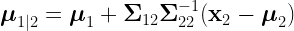
If the cognitive variables have the vector of particular values 

The conditional covariance matrix:
If we can assume multivariate normality, we can use these equations, to estimate the proportion of people with no scores below any threshold on any set of scores conditioned on any set of predictor scores. In this example, about 51% of people with scores of exactly 100 on all 14 cognitive predictors have no scores below 85 on the 9 academic tests. About 96% of people with this cognitive profile have no scores below 70.
Because there is an extremely large number of possible cognitive profiles, I cannot show what would happen with all of them. Instead, I will show what happens with all of the perfectly flat profiles from all 14 cognitive scores equal to 70 to all 14 cognitive scores equal to 130.

Here is what happens with the same procedure when the threshold is 70 for the academic scores:

Here is the R code I used to perform the calculations. You can adapt it to other situations fairly easily (different tests, thresholds, and profiles).
library(mvtnorm)
WJ <- matrix(c(
  1,0.49,0.31,0.46,0.57,0.28,0.37,0.77,0.36,0.15,0.24,0.49,0.25,0.39,0.61,0.6,0.53,0.53,0.5,0.41,0.43,0.57,0.28, #Verbal Comprehension
  0.49,1,0.27,0.32,0.47,0.26,0.32,0.42,0.25,0.21,0.2,0.41,0.21,0.28,0.38,0.43,0.31,0.36,0.33,0.25,0.29,0.4,0.18, #Visual-Auditory Learning
  0.31,0.27,1,0.25,0.33,0.18,0.21,0.28,0.13,0.16,0.1,0.33,0.13,0.17,0.25,0.22,0.18,0.21,0.19,0.13,0.25,0.31,0.11, #Spatial Relations
  0.46,0.32,0.25,1,0.36,0.17,0.26,0.44,0.19,0.13,0.26,0.31,0.18,0.36,0.4,0.36,0.32,0.29,0.31,0.27,0.22,0.33,0.2, #Sound Blending
  0.57,0.47,0.33,0.36,1,0.29,0.37,0.49,0.28,0.16,0.23,0.57,0.24,0.35,0.4,0.44,0.36,0.38,0.4,0.34,0.39,0.53,0.27, #Concept Formation
  0.28,0.26,0.18,0.17,0.29,1,0.35,0.25,0.36,0.17,0.27,0.29,0.53,0.22,0.37,0.32,0.52,0.42,0.32,0.49,0.42,0.37,0.61, #Visual Matching
  0.37,0.32,0.21,0.26,0.37,0.35,1,0.3,0.24,0.13,0.22,0.33,0.21,0.35,0.39,0.34,0.38,0.38,0.36,0.33,0.38,0.43,0.36, #Numbers Reversed
  0.77,0.42,0.28,0.44,0.49,0.25,0.3,1,0.37,0.15,0.23,0.43,0.23,0.37,0.56,0.55,0.51,0.47,0.47,0.39,0.36,0.51,0.26, #General Information
  0.36,0.25,0.13,0.19,0.28,0.36,0.24,0.37,1,0.1,0.22,0.21,0.38,0.26,0.26,0.33,0.4,0.28,0.27,0.39,0.21,0.25,0.32, #Retrieval Fluency
  0.15,0.21,0.16,0.13,0.16,0.17,0.13,0.15,0.1,1,0.06,0.16,0.17,0.09,0.11,0.09,0.13,0.1,0.12,0.13,0.07,0.12,0.07, #Picture Recognition
  0.24,0.2,0.1,0.26,0.23,0.27,0.22,0.23,0.22,0.06,1,0.22,0.35,0.2,0.16,0.22,0.25,0.21,0.19,0.26,0.17,0.19,0.21, #Auditory Attention
  0.49,0.41,0.33,0.31,0.57,0.29,0.33,0.43,0.21,0.16,0.22,1,0.2,0.3,0.33,0.38,0.29,0.31,0.3,0.25,0.42,0.47,0.25, #Analysis-Synthesis
  0.25,0.21,0.13,0.18,0.24,0.53,0.21,0.23,0.38,0.17,0.35,0.2,1,0.15,0.19,0.22,0.37,0.21,0.2,0.4,0.23,0.19,0.37, #Decision Speed
  0.39,0.28,0.17,0.36,0.35,0.22,0.35,0.37,0.26,0.09,0.2,0.3,0.15,1,0.39,0.36,0.32,0.3,0.3,0.3,0.25,0.33,0.23, #Memory for Words
  0.61,0.38,0.25,0.4,0.4,0.37,0.39,0.56,0.26,0.11,0.16,0.33,0.19,0.39,1,0.58,0.59,0.64,0.5,0.48,0.46,0.52,0.42, #Letter-Word Identification
  0.6,0.43,0.22,0.36,0.44,0.32,0.34,0.55,0.33,0.09,0.22,0.38,0.22,0.36,0.58,1,0.52,0.52,0.47,0.42,0.43,0.49,0.36, #Passage Comprehension
  0.53,0.31,0.18,0.32,0.36,0.52,0.38,0.51,0.4,0.13,0.25,0.29,0.37,0.32,0.59,0.52,1,0.58,0.48,0.65,0.42,0.43,0.59, #Reading Fluency
  0.53,0.36,0.21,0.29,0.38,0.42,0.38,0.47,0.28,0.1,0.21,0.31,0.21,0.3,0.64,0.52,0.58,1,0.5,0.49,0.46,0.47,0.49, #Spelling
  0.5,0.33,0.19,0.31,0.4,0.32,0.36,0.47,0.27,0.12,0.19,0.3,0.2,0.3,0.5,0.47,0.48,0.5,1,0.44,0.41,0.46,0.36, #Writing Samples
  0.41,0.25,0.13,0.27,0.34,0.49,0.33,0.39,0.39,0.13,0.26,0.25,0.4,0.3,0.48,0.42,0.65,0.49,0.44,1,0.38,0.37,0.55, #Writing Fluency
  0.43,0.29,0.25,0.22,0.39,0.42,0.38,0.36,0.21,0.07,0.17,0.42,0.23,0.25,0.46,0.43,0.42,0.46,0.41,0.38,1,0.57,0.51, #Calculation
  0.57,0.4,0.31,0.33,0.53,0.37,0.43,0.51,0.25,0.12,0.19,0.47,0.19,0.33,0.52,0.49,0.43,0.47,0.46,0.37,0.57,1,0.46, #Applied Problems
  0.28,0.18,0.11,0.2,0.27,0.61,0.36,0.26,0.32,0.07,0.21,0.25,0.37,0.23,0.42,0.36,0.59,0.49,0.36,0.55,0.51,0.46,1), nrow= 23, byrow=TRUE) #Math Fluency
WJNames <- c("Verbal Comprehension", "Visual-Auditory Learning", "Spatial Relations", "Sound Blending", "Concept Formation", "Visual Matching", "Numbers Reversed", "General Information", "Retrieval Fluency", "Picture Recognition", "Auditory Attention", "Analysis-Synthesis", "Decision Speed", "Memory for Words", "Letter-Word Identification", "Passage Comprehension", "Reading Fluency", "Spelling", "Writing Samples", "Writing Fluency", "Calculation", "Applied Problems", "Math Fluency")
rownames(WJ) <- colnames(WJ) <- WJNames

#Number of tests
k<-length(WJNames)

#Means and standard deviations of tests
mu<-rep(100,k)
sd<-rep(15,k)

#Covariance matrix
sigma<-diag(sd)%*%WJ%*%diag(sd)
colnames(sigma)<-rownames(sigma)<-WJNames

#Vector identifying predictors (WJ Cog)
p<-seq(1,14)

#Threshold for low scores
Threshold<-85

#Proportion of population who have no scores below the threshold
pmvnorm(lower=rep(Threshold,length(WJNames[-p])),upper=rep(Inf,length(WJNames[-p])),sigma=sigma[-p,-p],mean=mu[-p])[1]

#Predictor test scores for an individual
x<-rep(100,length(p))
names(x)<-WJNames[p]

#Condition means and covariance matrix
condMu<-c(mu[-p] + sigma[-p,p] %*% solve(sigma[p,p]) %*% (x-mu[p]))
condSigma<-sigma[-p,-p] - sigma[-p,p] %*% solve(sigma[p,p]) %*% sigma[p,-p]

#Proportion of people with the same predictor scores as this individual who have no scores below the threshold
pmvnorm(lower=rep(Threshold,length(WJNames[-p])),upper=rep(Inf,length(WJNames[-p])),sigma=condSigma,mean=condMu)[1]
In a previous post, I imagined that there was a gifted education program that had a strictly enforced selection procedure: everyone with an IQ of 130 or higher is admitted. With the (univariate) truncated normal distribution, we were able to calculate the mean of the selected group (mean IQ = 135.6).

Reading comprehension has a strong relationship with IQ 


Bivariate normal distribution truncated at IQ = 130
Here is the same distribution with simulated data points in 2D:

Expected values of IQ and reading comprehension when IQ ≥ 130
In the picture above, the expected value (i.e., mean) for the IQ of the students in the gifted education program is 135.6. In the last post, I showed how to calculate this value.
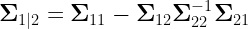
The expected value (i.e., mean) for the reading comprehension score is 124.9. How is this calculated? The general method is fairly complicated and requires specialized software such as the R package tmvtnorm. However in the bivariate case with a single truncation, we can simply calculate the predicted reading comprehension score when IQ is 135.6:
In R, the same answer is obtained via the tmvtnorm package:
library(tmvtnorm)
#Variable names
vNames<-c("IQ","Reading Comprehension")

#Vector of Means
mu<-c(100,100)
names(mu)<-vNames;mu

#Vector of Standard deviations
sigma<-c(15,15)
names(sigma)<-vNames;sigma

#Correlation between IQ and Reading Comprehension
rho<-0.7

#Correlation matrix
R<-matrix(c(1,rho,rho,1),ncol=2)
rownames(R)<-colnames(R)<-vNames;R

#Covariance matrix
C<-diag(sigma)%*%R%*%diag(sigma)
rownames(C)<-colnames(C)<-vNames;C

#Vector of lower bounds (-Inf means negative infinity)
a<-c(130,-Inf)

#Vector of upper bounds (Inf means positive infinity)
b<-c(Inf,Inf)

#Means and covariance matrix of the truncated distribution
m<-mtmvnorm(mean=mu,sigma=C,lower=a,upper=b)
rownames(m$tvar)<-colnames(m$tvar)<-vNames;m

#Means of the truncated distribution
tmu<-m$tmean;tmu

#Standard deviations of the truncated distribution
tsigma<-sqrt(diag(m$tvar));tsigma

#Correlation matrix of the truncated distribution
tR<-cov2cor(m$tvar);tR
In running the code above, we learn that the standard deviation of reading comprehension has shrunk from 15 in the general population to 11.28 in the truncated population. In addition, the correlation between IQ and reading comprehension has shrunk from 0.70 in the general population to 0.31 in the truncated population.
Among the students in the gifted education program, what proportion have reading comprehension scores of 100 or less? The question can be answered with the marginal cumulative distribution function. That is, what proportion of the red truncated region is less than 100 in reading comprehension? Assuming that the code in the previous section has been run already, this code will yield the answer of about 1.3%:
#Proportion of students in the gifted program with reading comprehension of 100 or less
ptmvnorm(lowerx=c(-Inf,-Inf),upperx=c(Inf,100),mean=mu,sigma=C,lower=a,upper=b)
The mean, sigma, lower, and upper parameters define the truncated normal distribution. The lowerx and the upperx parameters define the lower and upper bounds of the subregion in question. In this case, there are no restrictions except an upper limit of 100 on the second axis (the Y-axis).
If we plot the cumulative distribution of reading comprehension scores in the gifted population, it is close to (but not the same as) that of the conditional distribution of reading comprehension at IQ = 135.6.

Marginal cumulative distribution function of the truncated bivariate normal distribution
Imagine that in order to qualify for services for intellectual disability, a person must score 70 or below on an IQ test. Every three years, the person must undergo a re-evaluation. Suppose that the correlation between the original test and the re-evaluation test is 
pmvnorm function from the mvtnorm package (which is a prerequiste of the tmvtnorm package and this thus already loaded if you ran the previous code blocks).
library(mvtnorm)
#Means
IQmu<-c(100,100)

#Standard deviations
IQsigma<-c(15,15)

#Correlation
IQrho<-0.9

#Correlation matrix
IQcor<-matrix(c(1,IQrho,IQrho,1),ncol=2)

#Covariance matrix
IQcov<-diag(IQsigma)%*%IQcor%*%diag(IQsigma)

#Proportion of the general population scoring 70 or less on both tests
pmvnorm(lower=c(-Inf,-Inf),upper=c(70,70),mean=IQmu,sigma=IQcov)

#Proportion of the general population scoring 70 or less on the first test but not on the second test
pmvnorm(lower=c(-Inf,70),upper=c(70,Inf),mean=IQmu,sigma=IQcov)
What are the means of these truncated distributions?
#Mean scores among people scoring 70 or less on both tests
mtmvnorm(mean=IQmu,sigma=IQcov,lower=c(-Inf,-Inf),upper=c(70,70))

#Mean scores among people scoring 70 or less on the first test but not on the second test
mtmvnorm(mean=IQmu,sigma=IQcov,lower=c(-Inf,70),upper=c(70,Inf))
Combining this information in a plot:
 Thus, we can see that the multivariate truncated normal distribution can be used to answer a wide variety of questions. With a little creativity, we can apply it to many more kinds of questions.
I have made an easy-to-use Excel spreadsheet that can simulate data according to a latent structure that you specify. You do not need to know anything about R but you’ll need to install it. RStudio is not necessary but it makes life easier. In this video tutorial, I explain how to use the spreadsheet.
This project is still “in beta” so there may still be errors in it. If you find any, let me know.
If you need something with more features and is further along in its development cycle, consider simulating data with the R package simsem.
I am grateful that we live in an age in which individuals like Yihui Xie make things that help others make things. Aside from his extraordinary work with knitr, I am enjoying the ability to make any kind of animation I want with his animation package. My introductory stats lectures are less boring when I can make simple graphs move:

Correlations
 library(Cairo)
 library(animation)
 library(mvtnorm)
 n <- 1000  #Sample size
 d <- rmvnorm(n, mean = c(0, 0), sigma = diag(2))  #Uncorrelated z-scores
 colnames(d) <- c("X", "Y")  #Variable names
 m <- c(100, 100)  #Variable means
 s <- c(15, 15)  #Variable standard deviations
 cnt <- 1000  #Counter variable
 for (i in c(-0.9999, -0.999, seq(-0.995, 0.995, 0.005), 0.999, 0.9999,
    0.999, seq(0.995, -0.995, -0.005), -0.999)) {
 Cairo(file = paste0("S", cnt, ".png"), bg = "white", width = 700,
    height = 700)  #Save to file using Cairo device
 cnt <- cnt + 1  #Increment counter
 rho <- i  #Correlation coefficient
 XY <- matrix(rep(1, 2 * n), nrow = n) %*% diag(m) + d %*% chol(matrix(c(1,
    rho, rho, 1), nrow = 2)) %*% diag(s)  #Make uncorrelated data become correlated
 plot(XY, pch = 16, col = rgb(0, 0.12, 0.88, alpha = 0.3), ylab = "Y",
    xlab = "X", xlim = c(40, 160), ylim = c(40, 160), axes = F,
    main = bquote(rho == .(format(round(rho, 2), nsmall = 2))))  #plot data
 lines(c(40, 160), (c(40, 160) - 100) * rho + 100, col = "firebrick2")  #Plot regression line
 axis(1)  #Plot X axis
 axis(2)  #Plot Y axis
 dev.off()  #Finish plotting
 }
 ani.options(convert = shQuote("C:/Program Files/ImageMagick-6.8.8-Q16/convert.exe"),
    ani.width = 700, ani.height = 800, interval = 0.05, ani.dev = "png",
    ani.type = "png")  #Animation options
 im.convert("S*.png", output = "CorrelationAnimation.gif", extra.opts = "-dispose Background",
    clean = T)  #Make animated .gif
Here is a static image of a multidimensional scaling of the WAIS-IV and WIAT-III. It is interactive when you click it (Works best in Firefox & Chrome, not in IE or Safari).

Following the same procedures as I did with the WJ III, I have made an interactive 3D MDS of the WISC-IV. The image below is static but if you click it, you can rotate and zoom the image interactively.

WISC-IV MDS
I have been playing around with interactive 3D images (with the rgl package in R) and thought that it would be fun to present a multidimensional scaling (MDS) of the WJ III NU. Kevin McGrew has produced a number of beautiful images with MDS. My favorite is this one, not just because it is gorgeous, but because of the theoretical insights it communicates.
I simply took the correlation matrix from the WJ III NU standardization sample (ages 9 to 13) and subtracted each correlation from 1 to produce a distance measure. I performed classic MDS in R with the cmdscale function, allowing 3 dimensions. I colored each test with my guess as to which CHC factor it belongs.
If you click the static image below, you can play with it (Firefox and Chrome worked for me but Internet Explorer and Safari did not.):

WJ III MDS in 3D
Very cool!
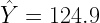
I recently was reading the book “Functional Art” and came across the work of Stefanie Posavec. Her Sentence Drawings (click here to see and click here to learn) caught my attention. Here is a ggplot2 rendition:

From what I understand about this visualization technique it’s meant to show the aesthetic and organic beauty of language (click here for interview with artist). I was captivated and thus I began the journey of using ggplot2 to recreate a Sentence Drawing.
I decided to use data sets from the qdap package.
Stefanie Posavec describes the process for creating the Sentence Drawing by making a right turn at the end of each sentence. I went straight to work creating an inefficient solution to making right hand turns. Realizing the inefficiency, I asked for help and utilized this response from flodel…
View original post 377 more words


